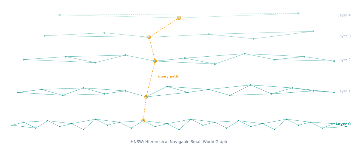
What Are HNSW Graphs? Hierarchical Proximity Search Explained

What Are HNSW Graphs?

HNSW stands for Hierarchical Navigable Small World. It is a graph-based data structure for approximate nearest neighbour (ANN) search: given a query vector, HNSW finds the k closest vectors in a large collection with high accuracy and very low latency. It is the dominant indexing algorithm used by production vector databases including Pinecone, Weaviate, Qdrant, and FAISS.

Without HNSW, finding the most similar vector to a query requires computing cosine or L2 distance to every vector in the collection. At 10 million vectors, this brute-force approach takes several seconds per query, making real-time retrieval impractical. HNSW reduces this to milliseconds by structuring vectors as a hierarchical graph and navigating it greedily.

The "Small World" part of the name refers to a property from network theory: in a well-constructed graph, any node can be reached from any other node in a small number of hops. The "Hierarchical" part refers to the multi-layer structure that makes this navigation efficient at scale.

How HNSW Graph Connectivity Affects AI Search Retrieval

AI search retrieval relies on HNSW or similar ANN indexes to retrieve candidate documents at query time. Understanding how the index is constructed reveals why content quality at the chunk level matters so much for AI search inclusion.

• Graph proximity reflects semantic proximity: Vectors for closely related content are connected in the HNSW graph. Content that occupies a dense cluster in vector space (many related documents nearby) will see its chunks connected to each other and retrieved together for relevant queries.
• Index coverage is not guaranteed for every chunk: HNSW only connects nodes that are nearby at construction time. A chunk that is semantically distant from all other corpus content will have poor graph connectivity and low retrieval probability. Producing content that relates to existing knowledge clusters improves retrieval chances.
• Chunking quality affects index structure: Semantic chunking produces chunks with tighter, more coherent vector embeddings. These chunks cluster better in the HNSW graph and are retrieved more reliably for relevant queries.
• AI search optimisation begins at the embedding layer: Our AI-driven SEO approach considers how content will be indexed and traversed in vector retrieval systems, not just how it will rank in traditional keyword search.

The Layered Graph Structure

HNSW organises vectors across multiple layers. The top layers contain a small fraction of all vectors, connected by long-range edges that span large areas of the vector space. The bottom layer (Layer 0) contains all vectors, connected by short-range edges to their nearest neighbours.

Each vector is assigned a maximum layer based on a random exponential distribution. A vector that appears in Layer 2 also appears in Layer 1 and Layer 0. The probability of being assigned to a higher layer decreases exponentially. In a graph with 1 million vectors, Layer 2 might contain only a few hundred nodes, while Layer 0 contains all 1 million.

The long-range connections at higher layers function as highways: they allow search to cross large portions of the vector space in a single hop. The dense local connections at Layer 0 allow precise refinement once the search has navigated close to the query region. This combination gives HNSW both coarse navigation speed and fine-grained precision.

How HNSW Search Works

HNSW search is a top-down greedy algorithm. It begins at a fixed entry point node at the highest layer and performs greedy descent: at each step, it moves to the neighbour of the current node that is closest to the query vector. When no neighbour is closer than the current node, it has reached a local minimum for that layer.

At this local minimum, the algorithm drops down one layer. At lower layers, the same node connects to more neighbours (the graph is denser), so greedy descent continues further. This process repeats until Layer 0, where the algorithm maintains a dynamic candidate list of the best candidates found so far and expands from them until no better options remain.

The result is a set of approximate nearest neighbours. The approximation error comes from the greedy descent: the algorithm may settle into a local minimum that is not the true global nearest neighbour. In practice, with appropriate parameters, HNSW achieves recall above 95% (meaning it finds at least 95 of the true 100 nearest neighbours) with query times under 5 milliseconds on commodity hardware, even for corpora with hundreds of millions of vectors.

Key Parameters

HNSW has three primary parameters that control its behaviour. All three are set at index creation time; changing them requires rebuilding the index.

• M (max connections per layer): Each node in Layer 0 maintains up to M connections to its nearest neighbours. Higher M means better recall and faster convergence in search, at the cost of more memory and slower construction. Typical production values are 16 to 64. Very high M (above 128) produces diminishing recall gains while index size grows linearly.
• ef_construction: The size of the dynamic candidate list maintained during graph construction. A larger value produces a better-quality graph (nodes connect to better neighbours) at the cost of slower indexing. Setting ef_construction below M produces a poor-quality graph. Typical values are 100 to 400.
• ef (query time): The dynamic candidate list size during search. Higher ef explores more of the graph before returning results, increasing recall at the cost of query latency. ef must be at least k (the number of results requested). Setting ef = k gives minimum latency at acceptable recall; setting ef to 2-4x k typically produces recall above 98%.

Where HNSW Is Used in Production Vector Databases

HNSW is the default or most widely used index type in every major vector database. It has largely replaced older approaches such as LSH (Locality Sensitive Hashing) and tree-based methods for high-dimensional dense vector search.

• Pinecone: Uses HNSW internally for its managed vector index with configurable M and ef_construction through the API.
• Weaviate: HNSW is the primary vector index. Weaviate also supports disk-based HNSW for large corpora that exceed RAM capacity.
• Qdrant: Uses HNSW with optional payload filtering that prunes the graph at query time based on metadata conditions.
• FAISS (Facebook AI Similarity Search): The open-source library includes HNSW as one of several index types, often used as the final re-ranking stage after IVF (Inverted File Index) pre-filtering.
• Elasticsearch and OpenSearch: Both support approximate k-nearest neighbour search using HNSW through the knn field type.

In practice, HNSW is used inside every system that performs RAG retrieval, semantic search, or similarity-based recommendation at scale. The Matryoshka embedding technique pairs naturally with HNSW: a low-dimension HNSW index handles coarse first-pass retrieval, and a full-dimension index re-ranks the candidates.

Frequently Asked Questions